• The assignment has 2 parts. The first is a pen-and-paper question. The second tries to get you familiar with the simulator you will be using for the programming assignment in Homework 2. You will be asked to run a few experiments and change some parameters.
• Part A involves material on A* search that will be covered in the lecture of Mon Sept 20th. However, you can read about A* in the book and start working on the question.
• Part B requires a certain startup time in order to get the simulator up and running as well as getting comfortable enough with it to set parameters and make minor changes. So please start early.
• NEW The exact experiments you need to run have been decided and are discussed towards the end of this page. We encourage you to install the simulator and make sure it is running, and read this document carefully to understand the various parameters involved.
• Homework 2 involves programming, so we encourage you to start thinking about it and maybe playing with the code if you finish Homework 1 early. The more time you devote to Homework 2 the better.

Part A: Question on A*

In A*, suppose that in addition to an admissible A* heuristic function h(n), you are told that there is a solution whose cost is K.

a) (8 points) How would you change A* to take advantage of this information (K) to reduce the number of nodes needed to be expanded, while maintaining optimality? Explain clearly all the changes.

Now instead of knowing K, suppose you are given a function H(n) that is an upper bound on the distance to the goal. That is, H(n) >= h*(n). Assume that h is monotone and that H (n) = infinity when there is no path to the goal.

b) (8 points) How would you change A* to take advantage of H (n) in order to reduce memory requirements, while maintaining optimality? Explain clearly all the changes.

c) (4 points) Will the proposed changes affect the number of nodes expanded? Explain.

d) (5 points) Is the assumption that h is monotone essential? Explain.

Part B: Familiarity with the simulator

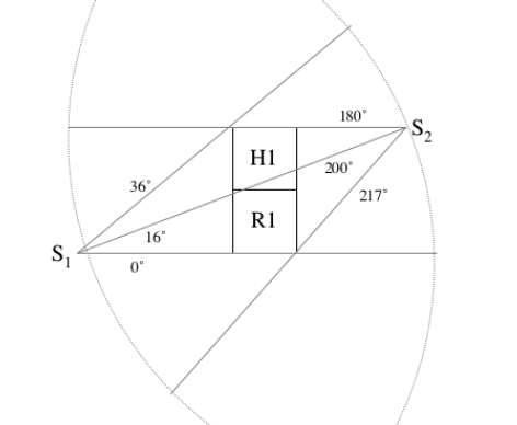
Your task is to get familiar with a variant of the radar scheduling problem called the setting-based resource allocation problem. In this problem, radars have multiple settings, each of which can be useful for multiple tasks. The resource allocation problem in this domain is to decide what setting to have each radar in, taking into account the needs of the various tasks, so as to maximize a global utility. For example, consider the following diagram from this paper.

In this diagram S1 and S2 are radars, H1 and R1 are tasks. The resource allocation algorithm would have to decide which of the following settings to have on the radars: 1) S1 sweeps over H1 and S2 sweeps over R1 (or vice versa) 2) Both radars sweep over either H1 or R1. 3) One or both radars sweep over an area encompassing both tasks. Example schedules are listed below:

Schedule 1:
S1 scans from 0-16 degrees with utility 5
S2 scans from 180-200 degrees with utility 3
Total Utility = 8

Schedule 2:
S1 scans from 0-16 degrees with utility 5
S2 scans from 200-217 degrees with utility 4
Total utility = 9

Schedule 3:
S1 scans from 0-360 degrees with utility 2
S2 scans from 180-200 degrees with utility 3
Total utility = 5

Schedule 4:
S1 scans from 0-360 degrees with utility 2
S2 scans from 0-360 degrees with utility 2
Total utility = 4 .
.
.

Schedule j:
S1 scans from 16-36 degrees with utiltiy 4
S2 does nothing
Total utility = 4

A brute force search algorithm (like Depth First Search (DFS)) will evaluate each of the potential schedules listed above and determine which is the most optimal. We hope to prune most of the schedules with a heuristic search like A*.

A task above is defined as an area of interest in the neighborhood of the radars. Each radar is able to scan a part of the task area for a certain duration. The utility gained is directly proportional to the time spent scanning the area of interest and the size of task area scanned. For simplicity in developing heuristics, the entire area of the task does not have to be scanned in order to gain a utility. If radars scan only a part of the area of interest a prorated utility is returned. For example if S1 scans from 0 to 8 degrees in Schedule 1 rather than scanning from 0 to 16 degrees, it would obtain a certain percentage of the utility gained by scanning from 0 to 16 degrees (a bit more than half, since it would be able to scan from 0 to 8 degrees for a relatively longer period of time).

A schedule determines settings for all the radars available to the system. To reduce the size of the search space, we will pre-prune those radar settings that do not scan over an available task. For example, S1 scanning from 36 to 50 degrees is not considered as a valid radar setting. The possible actions set (or settings) for each radar will be provided to you. You will be tasked with generating all possible schedules from those combinations. The simulator will also prune out all combination of actions that do not result in any utility (i.e. do not scan over a task area).

A formal representation of the problem is as follows:

• We have a set R = {S1,S2,S3...,Sm} that represents our radars.
• The set V_i = {a1,a2,a3....,an} represents the possible actions (or settings) for the radar i.
• The set T = {t1,t2,t3,...,tk} represents all the tasks.
• There exists a task utility function getValue(T_i, schedule) that defines the utility gained by the scanning schedule for task T_i.
• schedule is the scanning action for each radar.
• Each task has a getMaxUtil() that returns the maximum utility possible of this task.
• The number of potential schedules is approximately .

For this homework, you will be provided with:

• Simulator that generates and manages tasks and radars.
• DFS based search solution for scheduling radars.

Downloading and Installing the Source Code

Because of the trouble involved in setting up the simulator on many different machines that we faced in previous years, we ask you to install it on the edlab machines. We've tried the installation on the linux edlab machines (elnux1, elnux2, elnux3, elnux7) and can help you better if you use these machines. You can try to install it on another machine, but we may not be much help if problems arise. Please read more about edlab machine and use here. Note if you want to run this in windows, you will need to install and setup cgywin.

Your first step is to download and install the FARM simulation. There is Farm FAQ here .

• Copy the downloaded tar file to your directory on edlab
• Untar the file
• Download the script localfunctions.pl and put it under farm/lib (same directory as runfunctions.pl)
• Open the Makefile under the root farm directory and change the JAVART variable to point to the jdk folder on edlab.
• Make sure your JAVA_HOME is properly set and included in your PATH.
• Follow the instructions in the accompanying README file.

For the radar simulation:

• Download the radar simulation.
• Untar within the main farm directory.
• Change the first line in the radar/runradar script from

  require "../lib/runfunctions.pl";

  to

  require "../lib/localfunctions.pl";

• Follow the instructions in the corresponding README file to compile and run the radar simulation.

Once you have everything properly compiled, you should be able to run the simulation by running the "radar/runradar" script.

Details on Running the System

The Edlab linux machines are remote login only, meaning you're going to have to ssh to them. You will be running the simulator itself on the edlab machine and seeing the graphics on your local machine. To guarantee that graphics display properly, use the -XY options of ssh, so you do something like

ssh myname@elnux1.cs.umass.edu -XY

After ssh'ing into one of the elnux machines, you need to run the bash shell by typing bash.

Once you have the radar simulator running you should see two windows pop up. The first window

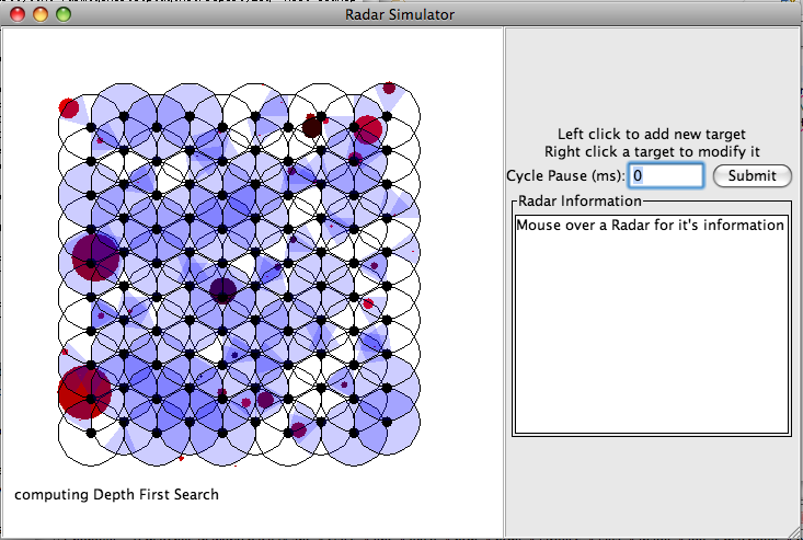
displays the radars and their current scanning action. Use this window primarily to visualize the task and radar locations. The second window

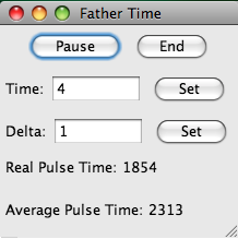
keeps time. A task is defined in this system as a target. Additional targets can be added by left clicking within the "Radar Simulator" window.

As the system is running the DFS algorithm logs its performance in the "search.output.log" file. An example log is as follows:

------- New Time Step -------
DFS's PROFILE: searched 449195 in 169323ms for the best value 20.2790020077377

In the above example, there were 3 radars and 10 tasks. There were about 450000 potential schedules to search from, with the optimal schedule providing a utility of about 21.

Configuring the simulator

The simulator can be configured from within RadarMetAgent.java. Here are some of the settings:

MAX_TIME - The total number of heartbeats for each trial.
radAgents - The number of radars
techniques[] - The search techniques you want to use have to be listed here
MAX_NUM_PHENOMENA[] - For each task, how many occerences of that task would you like to see? The tasks are listed right below.

If you add a new technique, you will have to do three things..

1. Add the name of your technique in the techniques[] list.
2. Add your technique in the usesConfigCorrect method in the RadarMetAgent class
3. Add your technique to the performCalculations method in the MCCAgent class

The search algorithm will be defined in the MCCAgent class. Look for searchWithDFS within for how to accomplish this.

Some other important files

MA0.log - This is where all the logged information gets saved

values.log - this is where all the performance information gets saved. What ends up in here is a combination of what is set to be logged within runradar and what is actually logged using setProperty

/src/farm/radar/plugins/RadarMetAgent.java - controls everything. Most of the important information about how things work in the simulator can be gained by examining what gets called from pulseBegin() in this file

/src/farm/radar/agent/MCCAgent.java - represents an individual scheduling agent

Experiments

Please answer the following questions and run the necessary experiments. All experiments should use the number of radars already specified in the code (3 radars). You only need 1 meta-agent.

1. Which part of the code is responsible for calculating the value of a node in the DFS search tree? Mention the name of the class and the method.
2. Which part of the code is responsible for generating the successor of a node in the DFS search tree? Mention the name of the class and the method.
3. In this question, you will investigate the behavior of DFS in terms of attained solution quality versus time (or effort). For 3 DFS searches:
   • Output the node number and the maximum schedule utility obtained so far. Because DFS will typically search hundreds of thousands of nodes, you want to do this every 1000 or 5000 nodes.
   • Plot the node number on the x-axis vs max utility on the y-axis. You can output any information you want with a normal System.out.println statement. You can then copy the results to a file and plot them using your favorite software.
   • Estimate the fraction of the nodes that would have been pruned had DFS recognized the optimal solution when it encountered it. E.g., if an optimal solution were obtained after exploring 100 nodes in a 300 node tree, 2/3 of the nodes would have been pruned).

Remember that :

• In each pulse, a DFS search is done to solve the scheduling problem.
• MAX_TIME in RadarMetAgent.java gives the number of pulses the simulation runs for.

Final Notes

Any comments, questions and bug reports are welcome.

When either one of us gets questions, we shall post them on the Q&A page. Please check it regularly.